Fort Collins Smoke Forecast 10/25/2016 (example not real, no data)

We are nearing the end of the wildfire season and today's forecast shows it. Lets take a look at the locations of the fires the NOAA Hazard Mapping System has determined to be producing significant amounts of smoke.

 This map shows there are no fires near Fort Collins. This should mean good news for local particulate matter (PM) pollution levels.

The figure below shows the 24-hour rolling mean PM2.5 (particles less than 2.5 micrometers in diameter) concentrations in Fort Collins. The plot is shaded using the EPA Air Quality Index. When the black line is in the blue shaded region the air quality is good, the tan area is classified as moderate.

The low concentrations of PM2.5 indicate that Fort Collins is not currently being influenced by smoke. With little to no fire activity nearby or upwind we can expect smoke free conditions today. 

Wildland fire and air quality data sources

In this post I will outline some of the resources I use when I am trying to understand the wildfires and resulting air quality impacts in my area. My hope is that this post be a one stop shop of resources for people concerned about wildfires.

The first thing I want to know is where fires are located. There are two means of obtaining fire locations. 1) Automated satellite based detection tools. 2) Human generated reports of fire locations. The weakness of the first is that satellites generally only detect large fires and have resolution limits that can limit the utility of the perimeter information provided. The weakness of the later is humans only detect fires where there are humans. The upshot of this is that these are often the fires we who recreate or own homes in the wildland urban interface (WUI) care most about.

First look, USGS wildfire GeoMAC mapping tool: Provides near real time fire perimeter data using both satellite and from incident intelligence sources. The interface has active fire, past fire, and fire boundary data layers that can be displayed on satellite imagery or topographic maps. Fire incidents can be clicked on to get basic information like name of fire and area burned. The map is easy enough to use but behaves differently than Google Maps (for some reason?) so there is a bit of a learning curve for most users. 

Incident Information System:
After I have identified the fires that are of interest to me I usually head over to http://inciweb.nwcg.gov/ for more detailed information. In the top right corner of the homepage, there is an incident scroll down menu. Scroll down and select the fire you want to learn more about.
If you are monitoring a fire that may pose a risk to you or your property this is probably the most valuable website to keep an eye on. Inciweb provides road closure and evacuation notices, evacuation shelter locations, projected fire activity, planned actions by fire agencies, and up to date fire perimeter .kml files (for viewing in Google Earth). This information is updated regularly for large fires. Unfortunately information for small fires can be slow to update or not available (but lets just remember that these agencies have limited resources).

Table 1: Example of Basic Information summary table provided by inciweb for the Wolverine Fire in Washington State. Screen shot from Monday 8/14/2015.   

Air quality alerts:

To find out if an air quality alert is in affect in your area go to weather.gov. The homepage will show a map of the US and current alerts issued by county. 

From the map you will be able to see if any significant weather or air quality alerts are in affect where you live. You can either click on your county on the map or enter your city and state in the search bar on the left side of the page (recommended). If there is an air quality alert where you live there will be a special alert bar at the top of the page after you enter your city and state. 

The alert bar will look like this. 

Click on the link for detailed information about air quality and recommended precautionary actions. If you prefer looking at more user friendly websites or a smartphone application that provides this information wunderground.com and their associated applications posts alerts made by the National Weather Service. Many popular smart phone applications (looking at you iphone default "weather" app) do not provide this information. So if the weather application you use does not show you an air quality alert that does not mean there isn't one! 

Past and real time air quality monitoring data:

Sometimes smoke can affect air quality and have adverse health affects before the Weather Service issues a warning (or any mention of smoke) in the standard forecast webpage. Because of this shortfall I like to check a new air quality monitoring system available from the US Forest Service AirFire team. http://smoke.airfire.org/monitoring/#/ allows easy access to particulate matter (smoke particle concentrations) monitoring data near you. Simply click on a monitor nearest you and select the "Use AQI Colors" to put the concentrations into context.

Example of output from the AirFire monitoring display system.  Screen shot taken 8/24/2015.

Washington State University Smoke Forecast:
WSU provides daily smoke forecasts for ID, OR, and WA. This is a remarkable achievement given the complexity of each step involved in trying to make a smoke forecast. Below is a simplified list of what needs to be done to produce a smoke forecast.

1. Fuel data. Trees, grass, shrubs, and different species of each emit different gasses and particles when burnt. In order to have an idea of what is put into the air when an area of land burns you need to know what burned and what type of emissions the fuel produces.
2. Fire data. Once you know the amount and composition of the smoke a given acre of land will produce when it is burned you need to know what is actually burning. To get at an amount of smoke in the air you multiply burn area by the expected emissions for a given acre of land.
3. Computer simulations. At this point we have a good idea of what gasses and particles will be emitted by a given fire. The pathway of that smoke is predicted using high resolution weather forecasts. The evolution of the particles and gasses within a smoke plume are computed using a model that accounts for the chemical and physical processes within a smoke plume. 

Combining these steps using state of the science technology enables the prediction of smoke concentrations. The WSU AIRPACT system uses the UW high resolution WRF weather model combined with the EPA Community Model for Air Quality (CMAQ) to predict the concentration of particles (number/volume) with a diameter less than 2.5 microns (referred to as PM2.5). The system is still under development but is currently working remarkable well. 

Sample of the smoke forecast visible product available from WSU. 

NASA MODIS visible satellite imagery: 

MODIS is a polar orbiting (orbits Earth generally passing near the poles) NASA satellite that provides daily images of the US lower 48. This resource provides an appreciation for the spatial scope smoke from fires can have. Air quality analysis use these images to assist them in deciding where to issue air quality warnings. The images are also stunning.

Visible image taken by NASA MODIS satellite on 8/24/2015. Areas of grey in the Northwest and extending along the Rocky Mountains through Colorado are from wildfire smoke. 

NOAA Hazard Mapping System Fire and Smoke Product

• Fire location analysis available in jpeg kml. 
• Good resource to find nice satellite loops for visible geostationary and polar orbiting imagery.

Humans vs. climate change. What starts more fires?

The EPA is interested in quantifying what future particulate matter (PM) concentrations might be in the future. In the U.S. intermountain west both extreme PM events and background PM concentrations are closely linked to wildfire activity. Once you start digging through fire science or air quality literature you don't get far before someone mentions the expectation that wildfire occurrence and area will increase with climate change. This of course makes sense, as the West warms and dries it is perfectly reasonable to expect the number of wildfires to increase (and this has been shown in many studies). However, humans have a much more direct and complicated relationship with fire than warming the planet by pumping green house gasses into the atmosphere. Other major ways we interact with fires include: 1) Fighting them. Depending on where a fire is located we don't let them burn without a fight. 2) Land management including fuel reduction, logging activity, and controlled burns. 3) We start them! There are of course other ways we interact with fire and earth system but I want to focus on the third one I just mentioned. Humans start a lot of fires. How many fires? I decided to take a look at the data to start to get an idea of what the human contribution is.

 

This clearly shows that humans do our fair share or starting fires. Smokey the Bear must be devastated. This figure includes all 50 states in the U.S. If we subset the data to include only western states it seems likely that Natural could start to close the gap with humans.

We have seen that humans start a lot of fires, more than nature does. How many acres of burned land are we responsible for?

 

I was hoping humans weren't going to be the leader in this category as well. These two figures combined seems to suggest that humans start a lot of fires but the fires we do start are generally small. It is also possible that a small number of fires for each start type account for a large fraction of total burned area.

Lets transition to looking at only western states. The states included in the following plots are Washington, Idaho, Nevada, Utah, California,
Montana, Oregon, Colorado, and Wyoming. First lets reproduce the two plots limited to data from these states.

In the western states there are more natural causes of fires than humans. This makes sense now that we are in the more arid, mountainous part of the country, where there are far fewer people than the more densely populated eastern States. The area burned by natural fires is about double that of human started fires. What do the burn area totals look like if we look at the data on an annual basis?

 

Lets look at the exact same data but in cumulative form.

 

The take home message is humans are responsible four A LOT of burning. When worrying about future PM emissions from fire it seems inappropriate to focus purely on the impact of climate change. Fires started by humans should be considered low hanging fruit in any effort to reduce burn area and the (somewhat) proportional emissions that follow.

R code and data used to make plots provided below

# load libraries
library(ggplot2)
library(sp)
library(rgdal)
library(rgeos)

# Data : http://wildfire.cr.usgs.gov/firehistory/data/fh_all.zip
# metadata : http://wildfire.cr.usgs.gov/firehistory/data.html

# Download the data
localDir <- getwd()
url <- 'http://wildfire.cr.usgs.gov/firehistory/data/fh_all.zip'
file <- paste(localDir, basename(url),sep='/')
if (!file.exists(file)) {
 download.file(url, file)
 unzip(file,exdir=localDir)
}

# create a layer name for the shapefiles (text before file extension)
layerName <- "firehistory_1980_2013_allagencies"

localDir <- "firehistory_1980_2013_allagencies"
# read data into a SpatialPolygonsDataFrame object
dataProjected <- readOGR(dsn=localDir, layer=layerName)

# Could use names(data_projected@data) or just:
names(dataProjected)

# Ok lets find out what burn area can be attributed to each of the start types
# first lets show the three catigories total count
cause <- dataProjected$CAUSE
naturalMask <- cause == "Natural"
humanMask <- cause == "Human"
NAMask <- is.na(cause)
 
nNatural <- sum(naturalMask, na.rm=TRUE)
nHuman <- sum(humanMask, na.rm=TRUE)
nNA <- sum(NAMask)

png(filename="fireStart.png")
par(las=1)
height = c(nHuman,nNatural,nNA)
barplot(height,
 names.arg=c("Human","Natural","unkown"),
 col="blue")
title("Cause of wild fires in U.S. 1980 - 2013")
dev.off()


burnArea <- dataProjected$TOTALACRES
humanArea <- sum(burnArea[humanMask], na.rm=TRUE)
naturalArea <- sum(burnArea[naturalMask], na.rm=TRUE)
NAArea <- sum(burnArea[NAMask], na.rm=TRUE)

png(filename="burnAreaAttributed.png")
par(las=1)
height = c(humanArea,naturalArea,NAArea)
barplot(height,
 names.arg=c("Human","Natural","unkown"),
 col="blue")
title("Total acres burned by cause of wild fires, U.S. 1980 - 2013")
dev.off()


# TODO: Show these catigories as total by year over time


# The next natural step is to do the same thing only for a subset of states we 
# are interested in

# states of interest, we want to create a mask where dataProjected is TRUE
# for any of these states
states <- dataProjected$STATE
statesOfInterest <- c("Washington","Idaho","Nevada","Utah","California",
 "Montana","Oregon","Colorado","Wyoming")

stateMask <- rep(FALSE,length(states))
for (state in statesOfInterest){
 stateMask[state == states] <- TRUE
}


dataProjectedSubset <- dataProjected[stateMask, ]


# Ok lets find out what burn area can be attributed to each of the start types
# first lets show the three catigories total count
cause <- dataProjectedSubset$CAUSE
naturalMask <- cause == "Natural"
humanMask <- cause == "Human"
NAMask <- is.na(cause)

nNatural <- sum(naturalMask, na.rm=TRUE)
nHuman <- sum(humanMask, na.rm=TRUE)
nNA <- sum(NAMask)

png(filename="fireStartWest.png")
par(las=1)
height = c(nHuman,nNatural,nNA)
barplot(height,
 names.arg=c("Human","Natural","unkown"),
 col="blue")
title("Cause of wild fires in U.S. western states 1980 - 2013")
dev.off()


burnArea <- dataProjectedSubset$TOTALACRES
humanArea <- sum(burnArea[humanMask], na.rm=TRUE)
naturalArea <- sum(burnArea[naturalMask], na.rm=TRUE)
NAArea <- sum(burnArea[NAMask], na.rm=TRUE)

png(filename="burnAreaAttributedWest.png")
par(las=1)
height = c(humanArea,naturalArea,NAArea)
barplot(height,
 names.arg=c("Human","Natural","unkown"),
 col="blue")
title("Total acres burned by cause of wild fires")
title(line=0.5, "western states 1980 - 2013")
dev.off()

# loop through years to see how area burned can be attributed over time
endDate <- as.POSIXlt(dataProjectedSubset$OUTDATED, format="%Y/%m/%d")

naturalAreaBurned <- rep(NA, length(1980:2013))
humanAreaBurned <- rep(NA, length(1980:2013))
NAAreaBurned <- rep(NA, length(1980:2013))

# Loop through and count total area burned for each
years <- 1980:2013
for (i in 1:length(years)){
 year <- years[i]
 yearMask <- (endDate$year+1900) == year 
 
 # count the years total burn by start type
 naturalAreaBurned[i] <- sum(burnArea[naturalMask & yearMask], na.rm=TRUE)
 humanAreaBurned[i] <- sum(burnArea[humanMask & yearMask], na.rm=TRUE)
 NAAreaBurned[i] <- sum(burnArea[NAMask & yearMask], na.rm=TRUE)
}

png(filename="acreasBurnedTimeSeries.png")
par(mgp= c(3, 1, 0))
plot(years, naturalAreaBurned, col="black", pch=19,
 ylab="acres",
 xlab="Year")

lines(years, naturalAreaBurned, col="black")
points(years, humanAreaBurned, col="red", pch=19)
lines(years, humanAreaBurned, col="red")
points(years, NAAreaBurned, col="magenta")

legendText <- c("Natural", "Human", "unknown")
legend("topleft", legend=legendText,
 col=c("black","red", "magenta"),
 pch=c(19,19,1),
 cex=1.8
 )
title("Acres burned in the western states by fire cause")
dev.off()

humanAreaCumulative <- cumsum(humanAreaBurned)
naturalAreaCumulative <- cumsum(naturalAreaBurned)
NAAreaAreaCumulative <- cumsum(NAAreaBurned)

png(filename="acreasBurnedCumulative.png")
par(mgp= c(3, 1, 0))
plot(years, naturalAreaCumulative, col="black", pch=19,
 ylab="acres",
 xlab="Year")

lines(years, naturalAreaCumulative, col="black")
points(years, humanAreaCumulative, col="red", pch=19)
lines(years, humanAreaCumulative, col="red")
points(years, NAAreaAreaCumulative, col="magenta")

legendText <- c("Natural", "Human", "unknown")
legend("topleft", legend=legendText,
 col=c("black","red", "magenta"),
 pch=c(19,19,1),
 cex=1.8
)
title("Cumulative acres burned in the western states by fire cause")
dev.off()

Subversion for busy scientists

Sometimes it feels more productive to trudge through medial clean up tasks than it does to step back and assess the utility of your project's code and knowledge base's organizational scheme. Never thought about how to organize a project's code base? Is knowledge base a strange concept, something probably taken care of by the absurd storage size of your email inbox? If you answered yes to either of these patronizing questions this post is for you. 

In this post

1. Attempt to convince you that subversion can make your life easier
2. Walk you through installing the necessary software (easy don't worry!)
3. Show you how to set up a project using a free subversion repository from assembla.com
4. Go over the  basics of using subversion at the command line
5. Provide an alternative for those less comfortable  working at the command line by demonstrating how to use a popular OSX subversion client.

Why use subversion?

Because your busy. You want a way to track the progress of your project. You don't want code that you spent time, sweat, and tears on getting lost, out of date, or unknowingly mucked up by some undergraduate assistant (guilty). Subversion is a free software versioning and revision control system that can help if you have ever done any of the following:

• Made a change to code, realized it was a mistake and wanted to revert back.
• Lost code or had a backup that was too old.
• Had to maintain multiple versions of a product/project.
• Wanted to see the difference between two (or more) versions of your code.
• Wanted to prove that a particular change broke or fixed a piece of code.
• Wanted to review the history of some code.
• Wanted to submit a change to someone else's code.
• Wanted to share your code, or let other people work on your code.
• Wanted to see how much work is being done, and where, when and by whom.
• Wanted to experiment with a new feature without interfering with working code.
• Wanted to know exactly what  code and data produced a particular figure.
• Wanted to make your work more reproducible.

Complete thread  on StackOverflow where developers describe how subversion/version control changed their lives more than magic beans changed the life of Dr. Oz. 

But I'm a scientist not a software engineer!

I have never met a scientist who has not run into any of the scenarios listed above above. Copying directories and time stamping them is not the same as version control. This method is prone to errors. It also lacks the convenience offered by Subversion.

Getting started

You're busy, so my start up instructions will be brief but if you think reading about version control technology is the most exciting thing you can do indoors you can read many more details here.  

Getting subversion on your machine

Instructions vary depending on what type of machine you are using. If you work in a windows environment the best instructions are use Git, subversion is probably not the right version control tool for you.

For Mac users  using OSX > 10.6 version control can be installed two easy ways. 1) Download Xcode in the app store. This requires a free Apple developer user ID. Once Xcode is installed you still need to download "command line tools". After opening Xcode 4 or 5 click "Xcode" near the apple button and select "preferences". Click on the "Downloads" tab and install the command line tools. OSX versions 10.6 and older come with Subversion installed.

2) If you don't plan on using Xcode and aren't interested in the extra baggage, you can download the command line tools separately from Apple. Your Apple ID will be required to go to the download page. Scroll down the list until you find the Command Line Tools and download.

For Linux users:  Linux platforms come with Subversion installed. To confirm you have Subversion type at the command line

which svn

If subversion is installed it will show something like

/usr/bin/svn

If subversion is not installed (very unlikely) you can find your platform and download subversion here.

Terminology and work cycle using Subversion

Now that Subversion is installed and we are ready to set up a project lets go over some terminology and briefly describe the version control work flow.

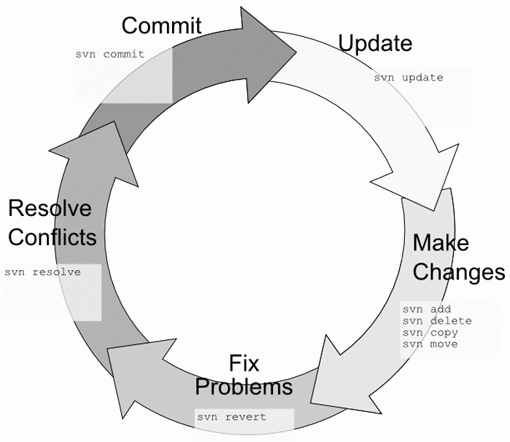
All of your files will be stored at a private URL, the location where this data is stored is the repository. The files that you first load to the repository and work on locally on your machine are called the local working copy. Each file will have a version associated with it. When you make changes to a file and want to move forward with those changes you commit that change and the version of the file in the repository will change. All versions of that file that have ever been committed will be saved in the repository.  When you make changes to the files in the repository by committing new code, collaborators will be able to update their local working copy to your latest version using update. If you or a collaborator see a mistake you made and don't like a new version that was committed you can revert to a previous version. If you and a collaborator both make changes to the same piece of code you will have to resolve differences between the two conflicting versions. Subversion offers a line by line comparison to make merging changes as easy as possible. More commands will be covered below.

Setting up a project

Subversion requires a repository. This is where all project files and versions are stored.  Its possible to use your own machine, or a machine in a local network but this post is for busy scientists not system administrators. The fastest way to get started is to use a free online repository by making a free account at assembla.com. Assembla is a secure Massachusetts based company that provides free (and paid) online Subversion repositories. It is also ridiculously easy to use. In June 2013 I got a group in the Atmospheric Sciences Department at the University of Washington to start using Subversion using an Assembla repository. You too can take this bold step!

To create a free account navigate to https://www.assembla.com/sign-up and sign up for a free account. The free account is limited to two collaborators, one project, and 500 MB of storage. When you get to step three make sure to choose the "Add a Subversion Repository" option. This web interface provides the perfect place to build a knowledge base for a project. Once your free account is set up and you are logged in, at the top of your project homepage you will see a menu that looks like this

• SVN: This tab is where your project code and files will live. We will populate this in a minute.
• Tickets: A place to document tasks required for your project. A great place to throw instructions you might have been given in an email or create a roadmap for a project
• Wiki: This is a good place to provide everything a collaborator might need to know about a project. Think of it as the three minute way to introduce a new user to a project. I like to include useful links, contact information, contracts/proposals.
• Messages: A place to post messages for all collaborators to see.
• Stream: Shows project activity, including changes to tickets and files. You can monitor what time changes are made, who is making changes, and what exactly they changed each time they committed code.
• Team: Where you add collaborators and change permissions.
• StandUp: A tool for creating project reports
• Files: Location where files not under version control can be uploaded and shared
• Admin: Change account settings, upgrade, delete, etc.

Under the SVN tab you will see the name of your project and a box next to it with a URL containing your project name. That URL is where all of your project files will live. The URL is password protected so only you and your invited teammates have access. The SVN tab starts with the standard Subversion organizational scheme of /trunk /tags and /branches directories.

• /Trunk Directory where you work on the latest copy of your project. This is where you and your collaborators will change files by "committing" code in your local working copy (explained in a minute).
• /tags This directory is where you save an instance or some state of a project. Say you are about to add a collaborator or make a major change to your code that could end up breaking things. Before these kinds of events you may want to "tag" the code. This will save the current state of the trunk at a unique URL under /tags (I will show you examples).
• /Branches Directory for the project when it starts to deviate from the original plan in the Wiki.

Time to fire up the terminal, we are going to use some svn unix commands to get started. To place an existing project in the Trunk we are going to use the svn import command. 

svn import /path/to/project/on/your/computer https://subversion.assembla.com/svn/YOURPOJECTNAME/trunk -m "Initial Import of existing project files."

You will see the files uploaded one at a time. The -m is to add a message to the commit. Subversion requires a message any time a change is made to the project URL. Now if you take a look at your Assembla SVN tab under trunk you will see all the files of your project. /path/to/project/on/your/computer is not a working copy. In order to start working on your project files under subversion you need to create a fresh working copy. To create a working copy you need to use the checkout command.

svn checkout https://subversion.assembla.com/svn/YOURPOJECTNAME/trunk

These files are under version control. Changes made to these files can be reflected in the repository trunk. Now we will go over the basic tools required to work on a project. The following instructions have been taken from http://svnbook.red-bean.com/. This website is an excellent resource for anyone planning on working with Subversion long term. Below is a slim and trim outline of the subversion work cycle as described by svnbook.

The typical work cycle using subversion looks something like this: 

Update your working copy. This involves the use of the svn update command. This command ensures that you are working on the latest version your projects files. If anyone else has made changes, or you made changes on a different computer this command will update your working copy to include the changes. Go to your local working copy directory and type

svn update # replaces copies of files on your computer with the latest version

Make your changes. The most common changes that you'll make are edits to the contents of your existing files. But sometimes you need to add, remove, copy and move files and directories—the svn add, svn delete, svn copy, and svn move commands mange those changes within the working copy.

# Create a test.txt file and save it in the trunk in order to test the following 
# commands

# Add the file
svn add test.txt

# To delete from the repository 
svn delete test.txt

# If you want to copy a file under version control and create a new one 
svn copy test.txt myTest.txt

# This is the same command you use to save a snapshot of the whole project by creating # a tag
svn copy https://subversion.assembla.com/svn/YOURPROJECTNAME/trunk \
https://subversion.assembla.com/svn/YOURPROJECTNAME/tags/v-0.0.1 -m "Saving the state 
of the project before I started using Subversion."

# Adding directories
svn mkdir Data

Review your changes. The svn status and svn diff commands are critical to reviewing the changes you've made in your working copy.

# You can see what changes you made to the project with the status command 
svn status

# svn status -v shows the status of all files, not just the ones with recent changes

On the off chance you make a change to a file that you don't like you can revert back to its previous state.

svn revert changedFile.text

Conflicts. A time may come when you run into version conflicts. If you make a change to a file that someone else is working on subversion will tell you about it.  You will need to integrate these changes in order to avoid a file getting out of date. In this scenario you may see something like the following after running svn update

Conflict discovered in 'test.txt'.
Select: (p) postpone, (df) diff-full, (e) edit,
        (mc) mine-conflict, (tc) theirs-conflict,
        (s) show all options: p
C    test.txt
Updated to revision 2.

# Your options

(e)  edit             - change merged file in an editor
(df) diff-full        - show all changes made to merged file
(r)  resolved         - accept merged version of file
(dc) display-conflict - show all conflicts (ignoring merged version)
(mc) mine-conflict    - accept my version for all conflicts (same)
(tc) theirs-conflict  - accept their version for all conflicts (same)
(mf) mine-full        - accept my version of entire file (even non-conflicts)
(tf) theirs-full      - accept their version of entire file (same)
(p)  postpone         - mark the conflict to be resolved later
(l)  launch           - launch external tool to resolve conflict
(s)  show all         - show this list

Publish (commit) your changes. The svn commit command transmits your changes to the repository where they create the newest versions of all the things you modified. Now when others update they will see these changes!

svn commit test.txt

Feeling a little lost or overwhelmed? Details for the work cycle outlined above can be found at http://svnbook.red-bean.com/en/1.7/svn.tour.cycle.html.

Using Subversion through a UI

Not everyone is comfortable working from the command line. For those of you who glazed over the previous section hopefully this will make up for it. There are many Subversion interfaces available. I will quickly show how to use a couple of the most popular.

Linux API

TortoiseSVN is the most popular interface for using Subversion on Linux platforms. 32 and 64 bit versions can be downloaded at http://tortoisesvn.net/downloads.html.

Mac Users API

Versions is a popular Subversion client for OSX. There is a free trial available for download at http://versionsapp.com/. If you fall in love with this sleek interface it can be yours for $59. After downloading, open Versions and click "New Repository Bookmark". 

A box with the following fields will appear

Enter the name of your project and the svn URL for location. Remember the location of your project can be found on your Assembla page under the svn tab. Don't forget to add trunk to this URL. Should look like https://subversion.assembla.com/svn/YOURPROJECTNAME/trunk. After you  "Create" your Repository bookmark all your files hosted at the project URL will be visible in Versions on the left hand bookmarks panel.

To create a local working copy of the project you need to check out the code. The checkout button is in the top left corner of the Versions frame. After you check out your project a new folder containing the local working copy will appear below the project bookmark in the left hand panel of the Versions window.

When changes are made to any files in the working copy a pencil will appear next to them under the "Browse" tab. You can commit the changes by the selecting the file and hitting the "Commit" button in the top left corner (next to checkout). The first time you commit a change you will be prompted to re-enter your Assembla username and password. All commands outlined in the previous basic workflow section are available in the Versions interface.  

Resources and Wrap Up